6. Exposure Assessment

Exposure via inhalation is estimated by calculating a time-weighted average air concentration (for example, mg/m³) for each receptor. More specifically, inhalation exposure concentration (EC) is expressed as an air concentration that is time-weighted over the duration of exposure for the receptor, reflecting the activity patternsThe activity or activities in which the receptor is assumed to be engaged involving details regarding where they are, when they were there, how long they were there, and over what area. of the specific receptor (USEPA 2009a).

Determining the appropriate values to use for each exposure factorFactors related to human behavior and characteristics that define the time, frequency, and duration of exposure; and help determine an individual's exposure to a chemical (USEPA 2011b). (such as exposure time, exposure frequency, and exposure duration) in a dose or exposure concentration equation can be complex, since in reality each of these exposure factors is not represented by a single value. These factors are most appropriately represented by a distributionA distribution describes the probability or likelihood of any potential value. of possible values because different individuals in the potentially exposed population will be exposed to varying degrees and for different periods of time. The range of values and the likelihood of any given value are characteristic of the behavior of different receptors.

Examples: Residential Drinking Water Exposure Scenario

For example, consider a residential drinking water exposure scenario. In order to estimate the amount of exposure to a particular chemical that a given resident might incur, the exposure duration must be determined (for example, years of exposure). Specifically, this exposure factor represents an estimate for how long people tend to live in one home before moving. According to USEPA (1997b), the 50^th percentile (the median) is 9 years and the 95^th percentile is 33 years (Figure 6-1).

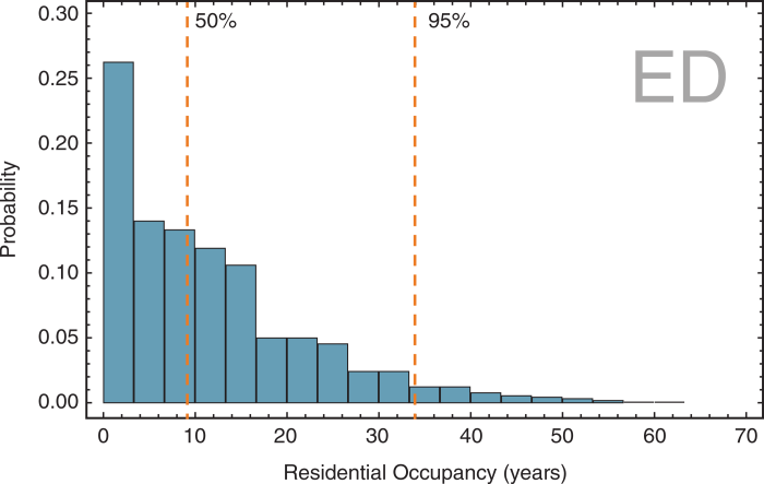
Figure 6-1. Probabilities of time spent living at one residence (exposure duration).

As with exposure duration, ingestion rate (L/day normalized by body weight) and exposure frequency (days/year) can also be appropriately represented by possible ranges of values rather than by single values (Figure 6-2 and Figure 6-3).

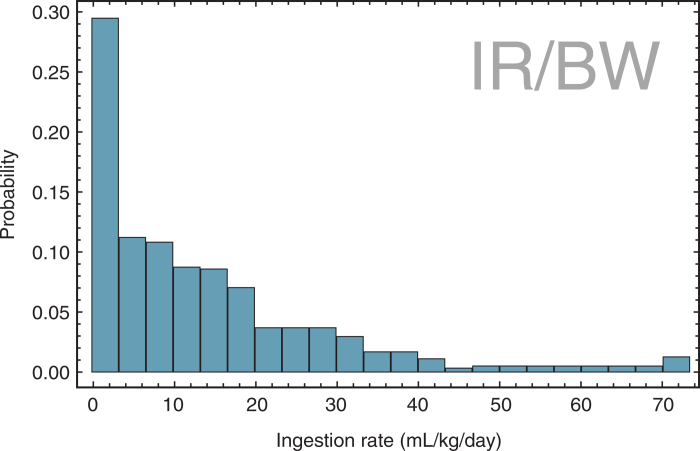
Figure 6-2. Drinking water ingestion rate probabilities (normalized by body weight).

 

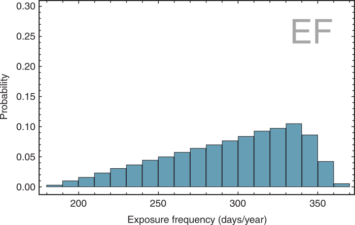
Figure 6-3. Exposure frequency probabilities.

These examples show that any exposure factor can be represented by many possible values covering a broad range (a distribution). As a result, quantifying a particular exposure for a potentially exposed receptor population does not yield a single result. The actual exposure (or intake) can be represented by a distribution of possible values, each with a different probability. This probabilistic analysis of environmental data can be performed using a Monte Carlo simulationA technique for characterizing the uncertainty and variability in exposure estimates by repeatedly sampling the probability distributions of the exposure equation inputs and using these inputs to calculate a range of exposure values (USEPA2001c)..

Example: Distribution Calculation – Monte Carlo Simulation

Continuing with the drinking water exposure scenario as an example, the distribution for the lifetime average daily dose (LADD) can be determined using the distributions above for ingestion rate (normalized by body weight), exposure frequency, and exposure duration. The resulting distribution for the exposure is shown in Figure 6-4.

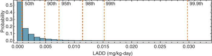
Figure 6-4. Drinking water exposure distribution for LADD.

While exposure factors are not represented by single numbers, most risk assessments use single values selected individually. Together, these values produce an estimate of exposure that is at the higher end of the range of plausible exposure values and ensure that the risk assessment is protective.

While exposure factors are represented most realistically as distributions rather than single numbers, for simplicity most exposure assessments use single values (a point estimate) from the distribution or range of possible values for each exposure factor. In some cases, these single values are often selected by regulatory agencies (typically referred to as “default exposure factors”) to produce an overall estimate of exposure that is at the higher end of the range of plausible exposures—an approach that is used to ensure that the resulting exposure assessment would be protective of human health. This higher end of the plausible range of exposure is typically referred to as the “reasonable maximum exposureThe highest exposure that is reasonably expected to occur at a site (USEPA 1989a)..” The reasonable maximum exposure (or RME) can be defined as “the highest exposure that is reasonably expected to occur at a site” (USEPA 1989a). More specifically, USEPA defines the RME as an exposure that falls within the 90^th percentile to 98^th percentile (USEPA 1992c); see Figure 6-5.

Figure 6-5. Reasonable maximum exposure.

The following sections discuss key issues encountered when determining appropriate exposure factors to use in calculating chemical exposure for a receptor. Options for addressing these issues are provided.

For receptor scenarios that are less frequently evaluated, certain default exposure factors (such as generic soil ingestion rates) are used in combination with other exposure factors that are based on site-specific or scenario-specific considerations (such as site-specific and receptor-specific exposure frequency and exposure duration). In these cases, the risk assessor must demonstrate that using site-specific exposure factors results in an overall exposure estimate that is still consistent with the concept of RME for the receptor scenario. Demonstration requirements can vary depending on the jurisdiction and individual regulatory agency. Some site-specific exposure factors may be justifiable based on professional judgmentDecisions made based on knowledge gained through education and experience., while others may require more detailed study, supporting data, and analysis. The summary data on human behaviors and characteristics that affect exposure to chemicals in the environment as presented in the Exposure Factors Handbook (USEPA 1997b; USEPA 2011c) are useful in determining and supporting site-specific exposure factors.

Consider whether using default exposure factors results in the calculation of RMEs that reflect the receptors and exposure pathways that are both currently occurring and that could reasonably occur (or be anticipated to occur) in the future. Many regulatory agencies prefer the use of default exposure factors when possible to ensure consistency in the management of potential health risks from site to site. Many risk assessments, however, require the estimation of exposure for receptors or exposure scenarios that are not routinely encountered. In these cases, default exposure factors may not be established. Site-specific factors may be used when default exposure factors are inconsistent with current and reasonably anticipated future receptors, and exposure pathways or default exposure factors are not available. The following sections provide options that can be used to justify the use of site-specific exposure factors.

6.1.1.1 Option – Collect Information to Justify Site-Specific Exposure Factors

Site-specific exposure factors can be developed by collecting information relevant to the behaviors and activities patterns of current and potential occupants of a site. Surveys can provide information regarding these patterns of potentially exposed receptors and can be performed during the site investigation process. Several methods can be used to perform surveys, including activity diaries and questionnaires (USEPA 1992c). Information can also be collected for site-specific activities from sources such as standard construction practices documentation or interviews with workers or other occupants of a site.

Activity diaries are used to gather specific information and data on the activity patterns of individual types of receptors, since they provide a sequential record of a person’s activities during specific periods of time. Typically these types of surveys can be performed over days or weeks. The individuals participating in the activity diary survey report all of their activities and locations for the period of the survey. When numerous participants are surveyed, forms must be carefully crafted for consistently tracking time and activities so that data generated by each individual is comparable.

Questionnaires can also be used to collect basic data regarding the activity patterns of individuals. The design of questionnaires can be a complex and detailed process and may require the help of professionals well-versed in survey techniques  (USEPA 1992c).

The information gained from survey studies such as activity diaries or questionnaires can be used either to develop site-specific exposure factors or to provide technical justification for site-specific exposure factors already developed. The use of a survey, however, and the information to be requested in the survey should be discussed in advance with the regulatory agency and other stakeholdersA stakeholder is anyone who has a “stake” in the development, outcome or decisions made as a result of a risk assessment. A stakeholder can be a person, a group, or an organization that is either affected, potentially affected, or has any interest in the project or in the project’s outcome, either directly or indirectly (Commission1997a; Commission 1997b; NRC 1996; NRC 2009). so that the data generated will be acceptable in the risk assessment. Additional discussion regarding the use of surveys can be found in Section 4.3.1 of USEPA’s Guidelines for Exposure Assessment (USEPA 1992c). Additional guidelines and information on survey techniques is provided in USEPA’s Survey Management Handbook (USEPA 1984).

6.1.1.2 Option – Using Institutional Controls or Engineering Controls to Justify Use of Site-Specific Exposure Factors

Most risk-based regulatory programs have provisions that allow for use of site-specific exposure factors, but using these assumptions can require institutional controlsNon-engineered instruments that help minimize the potential for human exposure to contamination and/or protect the integrity of the remedy (USEPA 2001c). Examples include deed restrictions on land use, groundwater use restrictions, and city ordinances prohibiting private well installations. The use of these controls typically require a specific mechanism for placing the restriction and future compliance with the restriction. The timing of the decision to use an institutional control, as well as, the specific mechanism to be used may be based on criteria outlined in statute, regulation, policy or guidance. or engineering controlsEngineered and constructed physical barriers to contain, prevent, or mitigate exposure to chemicals in an environmental medium. Examples of engineering controls include engineered caps and subslab depressurization systems, mitigation barriers, and fences. Similar to activity and land use restrictions, engineering controls also typically require a specific mechanism for noticing the presence of engineering control and related restrictions, as well as long-term maintenance and management of the control. The timing of a decision to use an engineering control, and the specific mechanism to be used, may be based on criteria outlined in statute, regulation, policy, or guidance. to ensure that the assumptions regarding exposure are maintained in the future.

Institutional controls (for example, deed restrictions or restrictive covenants) are legally binding and help to minimize the potential for exposure and protect the integrity of a risk managementThe process of identifying, evaluating, selecting, and implementing actions to reduce risk to human health and to ecosystems. The goal of risk management is scientifically sound, cost-effective, integrated actions that reduce or prevent risks while taking into account social, cultural, ethical, political, and legal considerations (Commission 1997a). action (USEPA 2012d). Institutional controls generally require the landowner or operator either to refrain from using land in a certain way or to proactively maintain and use the land only in a certain way (for example, disallowing residential land use, disallowing the use of groundwater for potable purposes, or maintaining an asphalt surface). Deed restrictions and restrictive covenants are also typically recorded with local land records.

Example: Using Institutional Controls to Justify Site-Specific Exposure Factors in a Commercial Facility

Consider a risk assessment in which indoor vapor intrusion exposure is evaluated as a current and reasonably expected exposure scenario. Assume that the occupied building in question is a commercial facility with two floors and a subgrade basement.

Currently, operations in this commercial building are mostly performed on the first floor and second floor, while the basement is only used for storage and utilities. Workers spend little time in the basement (generally no worker spends more than 1 hour each week in the basement). The risk assessment is performed assuming that the exposure time (ET) of any worker in the basement is 1 hour/week. The risk assessment also assumes that workers could be present in the first and second floor of this building for 40 hours/week. Vapor intrusion related exposure concentrations, in each of these exposure units (specifically, the basement and the first/second floor), are evaluated and the associated risks are shown to be acceptable. However, the conservative risk estimates for a worker’s exposure within the basement exposure unit are only 10 times below the acceptable risk management goal.

While the risk assessment demonstrates that current risks are acceptable given the described exposure conditions, in the future, if workers spend more time the basement (for example, 10 hours/week), then potential vapor intrusion exposure may exceed acceptable levels. In this case, an institutional control mandating that access to the basement be controlled to less than 10 hours/week could be used to support and justify the site-specific exposure factor used in the risk assessment. This approach would also provide assurances that acceptable risks are maintained in the future.

6.1.1.3 Option – Use Probabilistic Exposure Assessment to Justify Site-Specific Exposure Factors

Probabilistic exposure assessment is also a tool that can be used to support and justify site-specific exposure factors. As shown in Figure 6-5, RME represents exposures that would be at the high-end of the range of plausible exposures (within the 90^th percentile to the 98^th percentile exposure) (USEPA 1992c).

Developing probabilistic distributions for each individual exposure factor, for example using the data and information provided in the USEPA’sExposure Factors Handbook (USEPA 2011c), and then combining these distributions using Monte Carlo simulation as explained in Section 6.1, provides a way to understand the range and likelihood of possible exposures (see Figure 6-4 above). In particular, this method can be used to determine the exposure concentrations that would fall inside the RME range (between the 90^th to 98^th percentiles).

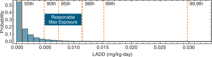
Figure 6-6. RME for residential drinking water exposure scenario.

As illustrated in Figure 6-6, the RME for residential drinking water would fall between about 0.005 mg/kg-day and about 0.012 mg/kg-day (based on a constant concentration of 1 mg/L in drinking water).

Example: Using Probabilistic Exposure Assessment to Justify a Site-Specific Drinking Water Exposure Factor

Consider the equation used to estimate the LADD for drinking water exposure. Assuming a constant chemical concentration of 1 mg/L and an averaging time equal to 70 years, point values for the remaining exposure factors can be justified by ensuring that they would result in a combined exposure that would fall inside the RME range noted above. For example, using generic default assumptions for an adult for ingestion rate (IR) = 2 L/day, exposure frequency (EF) = 350 days/year, exposure duration (ED) = 30 years, and body weight (BW) = 70 kg, would yield a LADD of 0.0117 mg/kg-day. This value falls at the top of the 0.005- 0.012 mg/kg-day RME range detailed above. Thus, the individual point values used for each exposure factor can be justified since, taken together, they yield an exposure that would represent an RME. Drinking water exposure is presented here as an example, because the exposure factors above are generic and routinely used in evaluating such exposures. A similar analysis and approach can be used to justify site-specific exposure factors when nonroutine exposure scenarios are encountered.

Probabilistic exposure assessment (USEPA 2001c) is infrequently used in risk assessment and may not be appropriate for all analyses. One limitation that may be encountered is whether data are available for exposure factors in order to develop the distributions similar to those shown in Figure 6-1 to Figure 6-3. Further information on probabilistic risk assessmentA technique that uses statistically derived distributions of input values (for example, exposure factors) to calculate a range of risk. for site risk assessments is available from USEPA (2001c). Another guidance document, A Review Article of Probabilistic Risk Assessment of Contaminated Land, defines remedial action objectives using probabilistic methods for the Superfund program (Oberg and Bergback 2013).

6.1.2.1 Option – Prorating Exposure Factors or Using a Fraction Contacted Exposure Factor

Prorating soil ingestion rates is appropriate on sites where multiple, separate exposure areas (or units) exist. If a worker is likely to spend equal time in each of these areas, then using a standard default soil ingestion rate as an exposure factor for each exposure areaA geographic area over which a receptor is reasonably assumed to move at random and equally likely to come into contact with an environmental medium (for example, soil) both spatially and temporally. An exposure area is further defined on the basis of observed or assumed patterns of receptor behavior, historic activity, and the nature and extent of chemicals in environmental media (USEPA1989a). An exposure area may also be called an exposure unit. could greatly overestimate the worker’s total exposure and associated risk. In this instance, it would be appropriate to prorate the daily soil ingestion rate (for example, 50 mg/day) across the multiple areas of exposure (for example, exposed to Area 1 50% of the time, Area 2 25% of the time, and Area 3 25% of the time). Thus, the worker’s total daily soil ingestion would still equal the default value soil ingestion value (25 mg/day + 12.5 mg/day +12.5 mg/day = 50 mg/day), but that value would be assumed to come from multiple areas within the site, each with potentially different degrees of contamination. Use of a fraction contacted (FC) exposure factor in evaluating the dose for each unique exposure area facilitates this approach.

With the proration of exposure factors, some regulatory programs may require institutional or engineering controls so that the final assumed exposure factors used in the exposure assessment are consistent with future land uses. For example, if it is assumed that a worker is exposed evenly to two different areas of a site, and the exposure assessment prorates the soil ingestion amount evenly between these two areas (for example, 25 mg/day and 25 mg/day), then the exposure assessment may not be protective when a worker is exposed to one of the areas for a greater period of time (for example, 75% in Area 1 and 25% in Area 2).

6.1.3.1 Option – Incorporate a Bioavailability Factor into the Exposure Equation

Where site-specific or media-specific data on bioavailability are known, the chemical exposure calculation (the potential dose) can be converted to an applied dose and internal dose by adding a bioavailability exposure factor (range: 0 to 1) to the dose equation.

The bioavailability factor should take into account: (1) the ability of the chemical to be extracted from the environmental mediumSoil, surface water, groundwater, indoor air, outdoor air, sediment, and other parts of the environment that may be impacted by the release of a chemical. (for example, soil); (2) the ability of the chemical to be absorbed into the body; and (3) other losses between ingestion and contact with the lung or gastrointestinal tract. When no data or information are available to indicate otherwise, the bioavailability factor is usually assumed to be 1 (USEPA 1992c). For example, ingestion of a metal adhered to soil may result in less absorption through the gastrointestinal tract than would occur if the metal were ingested in water or food. In this scenario, use of toxicity valuesDerived values (for example, reference doses and slope factors) that can be used to estimate the incidence or potential for adverse human health effects in receptor (USEPA 2015h). (for example, oral reference dose or slope factorAn upper bound, approximating a 95% confidence limit, on the increased cancer risk from a lifetime exposure to an agent. This estimate, usually expressed in units of proportion (of a population) affected per mg/kg-day, is generally reserved for use in the low-dose region of the dose-response relationship, that is, for exposures corresponding to risks less than 1 in 100 (USEPA 2013).) that were derived based on exposures to the metal in water or food would likely overestimate the calculated risks from ingestion of the metal in soil. USEPA (2007c) has published guidance on evaluating the bioavailability of metals in soil, specifically with regards human health risk assessment. USEPA has also published specific guidance for lead and arsenic, accounting for their relative bioavailability by including a bioavailability exposure factor (USEPA 2007c; USEPA 2007a; USEPA 2009d; USEPA 2012h).

6.2.1.1 Option – Establish Exposure Areas Based on Known or Anticipated Uses

When quantitatively evaluating exposure to chemicals in environmental media at a site as part of the risk assessment, consider the spatial distribution of chemical concentrations relative to the exposure scenario being evaluated. Assuming that potential exposure of receptors to chemicals can occur at any depth throughout the entirety of the site or investigation area may overlook alternatives to laterally or vertically refining the exposure area.

Such refinements could include:

1. Using different lateral exposure areas based on an understanding of differing activity patterns of different receptors at a site (for example, residents would be exposed only over half-acre areas, whereas construction workers would be exposed over the entire area).
2. Using different vertical exposures units that are relevant to the exposure scenario or pathway being assessed. For example, residential incidental ingestion, dermal contact, and particulate inhalation exposure to soil would commonly involve only contact with chemicals in surface soil, whereas construction workers or maintenance workers could be potentially exposed to chemicals in surface and subsurface soil (USEPA 1989a).

Establishing exposure areas that are designed to evaluate potential exposures is critical to understanding, using, and communicating the results of the risk assessment. Similarly, understanding inherent limitations of a risk assessment that results from the exposure areas evaluated is equally important to using and communicating the results in decision making. For example, risks calculated for a half-acre residential area many not be relevant if the area is further subdivided into smaller residential parcels in the future.

In general, exposure areas in the risk assessment should be based on the exposure scenarios defined in the CSM, and not on the investigational areas. Defining exposure areas based on activity patterns generally requires additional information on potential uses. The additional data are used to support the assumptions regarding potential uses and to support decisions made in calculating the average concentration.

6.2.1.2 Option – When Exposure Areas Cannot be Reasonably Established

Considering the spatial distribution of chemical concentrations relative to the exposure scenario is important in the exposure assessment, however, in cases where redevelopment is possible, information on the location and type of activities is not available. In these cases, certain exposure assessments might evaluate receptors by assuming equal likelihood of exposure across the entire site, or the assessment may be performed by comparing individual data points to cleanup criteria (for example, preliminary remediation goals). While these approaches may be conservative for some sites, they are not conservative for all.

When information on the location and type of future activities is not available, an alternative to the common approaches discussed above is to initially perform the exposure assessment using conservative assumptions regarding the size of hypothetical exposure areas for a given receptor. For example, start by assuming that every sampled location represents its own exposure area in which receptors will be exposed for their entire exposure frequency and exposure duration. This approach is analogous to comparing data to screening values and does not rely on areas that were identified based on historical releases or investigation to dictate future uses. Additionally, the initial definition of exposure areas based on activity patterns is not required. To illustrate this concept, the polygons on Figure 6-7 represent hypothetical exposure areas represented by each soil sample (specifically, each polygon is a hypothetical exposure area represented by the individual sample location).

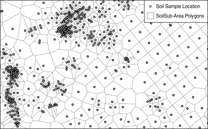
Figure 6-7. Soil sampling locations as individual exposure areas (represented by Thiessen polygons).

If the risks at each location are acceptable, then the risk assessment could conclude that the area represented by the boring location does not pose an unacceptable risk, regardless of how an actual future exposure area is eventually defined. Conversely, if the risks at certain locations are not acceptable, more realistic hypothetical exposure areas could be formed (for example, areas that consist of the initial location and adjoining locations to obtain a reasonable area where exposures could occur) to determine whether additional action would be warranted (Figure 6-8). Overall, this approach can help streamline the risk assessment by limiting the area over which difficult decisions regarding potential future activity patterns must be made.

Figure 6-8. Locations potentially warranting further assessment or risk management.

6.2.2.1 Option – Using Measured Data for the EPC

Measured concentrations may be helpful in characterizing the current average concentrations to which receptors will be exposed. In some cases, measured concentrations can be conservative estimates of future conditions (for example, current concentrations in soil versus future concentrations following leaching or volatilization) and may be appropriate for evaluating future receptors, especially when these conservative estimates of cumulative riskThe combined risks from aggregate exposures (combined exposure of an individual (or defined population) to a single chemical via relevant exposure routes, exposure pathways, and exposure media) to multiple chemicals (USEPA 2003c). are acceptable.

Using measured concentrations to estimate current EPCs is generally appropriate when exposure of a receptor involves direct contact with the medium (for example, direct exposure to chemicals in soil). Using measured concentrations is also generally appropriate when site monitoring data were collected directly at an exposure pointA location of potential contact between a receptor and a chemical (USEPA 1989a). (for example, a drinking water well or indoor air) (USEPA 1989a).

Measured concentrations may not be appropriate when concentrations measured over a short period are used to characterize a long-term exposure. For example, indoor air concentrations, obtained from a discrete sample collected over a relatively short period of time, would not be appropriate as the EPCs in a risk assessment evaluating chronic indoor exposure (25 or 30 years of exposure). These EPCs could overestimate or underestimate risks, since the measured concentrations over a short period (for example, 24 hours) generally do not characterize the long-term average exposure concentration. While the collection of samples over a longer period of time may help in understanding the variabilityA population’s natural heterogeneity or diversity, particularly that which contributes to differences in exposure levels or in susceptibility to the effects of chemical exposures (Commission 1997a). For example, workers may perform different functions that may affect time, frequency, and duration of contact with an environmental medium). Variability cannot be reduced by collection of additional data. in potential exposure with time, in many cases modeling EPCs may be more appropriate for long-term exposures.

6.2.2.2 Option – Using Modeled Exposure Concentrations for Determining the EPC

While measured concentrations of chemicals to determine the EPC may be helpful in understanding current conditions, these concentrations may not predict EPC over the entire exposure period (for example, use of short-duration indoor air monitoring data to evaluate and make decisions regarding long-term chronic vapor intrusion exposures).

Using modeled concentrations of chemicals to determine the EPC is useful for estimating future and long-term exposures to chemical concentrations in environmental media. EPCs derived from modeled concentrations can also be useful for estimating current or future EPCs in environmental media in areas where existing measured concentrations are unavailable (USEPA 1989a) or where measurements cannot be collected (for example, to evaluate vapor intrusion exposure into a future building). Finally, modeling concentrations can be used in conjunction with available site data from the source medium to estimate the change in concentrations over the exposure period (USEPA 1989a) for chemicals that degrade in the environment (for example, anaerobic dechlorination of tetrachloroethene in groundwater) or deplete over time (for example, volatilization from soil or leaching from soil to groundwater).

Specific instances where EPCs derived from modeled concentrations could be considered include the following:

• when the exposure being evaluated will occur in the future (for example, on- or off-site ambient air, off-site groundwater)
• when data regarding the change in chemical concentration over time is unavailable or lacking (for example, situations when chemical concentrations could change with time or when the collection of discrete samples over short periods of time can capture the potential variability in concentration over a longer period)
• when the collection of direct measurements would not be possible (for example, vapor intrusion sampling in areas where buildings do not currently exist but are planned in the future)
• when using measured concentrations is limited by the laboratory detection limit (for example, to predict concentrations of chemicals that may be present below quantitation limits, but which could still cause unacceptable site-related exposures)

Appendix C provides a list of models routinely used to calculate EPCs for different exposure scenarios and exposure pathways. The basis, derivations, details, assumptions, and limitations of these models are not discussed in this document, however, references and links to additional guidance are provided for each model.

6.2.3.1 Option – Use a Finite-Source Model

Using a finite-source modeling approach generally requires chemical concentrations to be well defined, which may require additional field information as compared to a standard, infinite source model. The additional field data are generally used to support necessary assumptions for finite mass calculations, for example, defining the vertical extent of volatile chemicals in vadose zone soil.

An example of a finite model used for outdoor inhalation exposure due to volatilization of chemicals from soil is the Jury model to estimate vapor flux from a finite soil source (Jury, Spencer, and Farmer 1983). This volatilization model estimates the flux of a chemical from either an infinite (the default approach used in calculating most criteria) or a finite soil source (USEPA 1996b). The finite source equations are shown in Section 3.1.1 of USEPA’s 1996 Soil Screening Guidance Technical Background Document (USEPA 1996b) The EMSOFT screening model is also available (USEPA 2002b), which is based on the work of (Jury, Spencer, and Farmer 1983).This program may be used to:

1. Determine concentrations of chemicals remaining in the soil over a given duration.
2. Quantify the mass flux (rate of transfer) of chemicals into the atmosphere over time.
3. Calculate chemical concentrations in air by inputting the mass flux values into atmospheric dispersion models (USEPA 2002b).

6.2.3.2 Option – Use a Mass Balance Check

The results from infinite source models in some cases (for example, equilibrium partitioning for chemical migration from soil to groundwater) can violate mass balance considerations (USEPA 1996c). To address this issue, incorporate a mass balance check when estimating the finite chemical mass that can infiltrate into groundwater. A mass balance check in the evaluation of soil migration to groundwater verifies that the assumed mass of a chemical migrating to groundwater over the assumed exposure period does not exceed an upper-bound estimate of the chemical’s mass in soil. The check can be performed by calculating concentrations in soil that would still result in acceptable risks even if the entire mass of contamination in the source area were to leach into groundwater over the exposure period.

If the chemical mass in soil is less than the mass to which a potential receptor could be exposed over the exposure period, then the exposure concentration would not be reached because there is insufficient mass in the soil to maintain the calculated drinking water concentrations using an infinite mass approach (Figure 6-9).

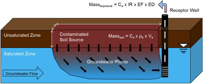
Figure 6-9. Soil migration to groundwater – mass limited check.

In these instances, the average concentration that would result over the exposure period, assuming all of the mass were to leave the source and migrate to the exposure point, could be used as a conservative upper-bound estimate of potential exposure over the exposure period.

6.2.4.1 Option – Use Upper Confidence Limits (UCL) on the Mean

The upper confidence limit (UCL)The upper boundary of a range of values. The range of values is referred to as a confidence interval. on the mean provides a conservative estimate of the average exposure concentration and accounts for uncertainties such as limited sampling data (USEPA 1992d). For example, the 95% UCL is the concentration at which only a 5% chance exists that the true mean of the data set would be higher. The more sampling data that is available, the closer the UCL should come to the true mean. In other words, fewer samples result in a higher UCL for the mean concentration and thus in higher potential risk or hazard.

UCLs can be calculated using a number of methods (for example, methods that assume the data are normal, lognormal, or gamma distributed, or the data are nonparametric and thus do not rely on the assumption of an underlying distribution). Software packages are available to perform UCL calculations. For example, USEPA’s ProUCL is a statistical software package (with graphical tools) that can calculate UCLs (USEPA 2013d).

The following issues and limitations should be considered when calculating UCLs on the mean:

• The fewer the number of samples, the greater the uncertaintyThe lack of perfect knowledge of values or parameters used in a risk assessment. Uncertainty may be reduced by collection of additional data. that the sample mean is representative of the true mean. These uncertainties result in large confidence limits around the mean and potential estimates of the mean that are biased high. Consider the benefit of collecting appropriate additional samples to increase confidence that the sample mean is more representative of the true mean.
• Compare the UCL result with the maximum detected or modeled concentration. If the calculated UCL is greater than the maximum detected concentration, then the maximum detected or modeled concentration should be used to estimate exposure concentrations (USEPA 1989a; USEPA 2002a). Statistical software such as ProUCL may recommend alternative computations if the UCL on the mean exceeds the observed maximum concentration (USEPA 2013e).
• Application of the UCL statistic assumes the sample collection locations are generally unbiased across the exposure area. In contrast, data collection for many site assessments focuses on the chemical source areas and areas of highest chemical concentrations to document the nature and extent of the chemical release. Thus, sampling locations are not often evenly distributed throughout and are biased within the exposure area. In these instances, the UCL on the mean concentration may also be biased high. Such high bias on the mean, while conservative, may not be suitable for use in a risk assessment if it excessively overestimates the risks. Other data analysis methods may provide better estimates of the true mean in these situations (see Section 6.2.4.2).

6.2.4.2 Option – Use Area-Weighted Averages

Area-weighted averages may be used to estimate appropriate exposure concentrations (Pedersen and LaVelle 1997; NJDEP 2012b) when exposure units are fairly well defined and when data for an exposure area are so unevenly distributed that UCLs on the mean do not provide reasonable estimates of the exposure concentration. For example, Figure 6-10 depicts a case in which a number of surface soil sample locations are clustered in one corner of the exposure area. The sample concentrations (mg/kg) are depicted in the figure. These cases typically arise from focused sampling of a small area in which many samples with high concentrations are clustered. In this example, this distribution could result in a significant overestimate of the mean concentration in an exposure area.

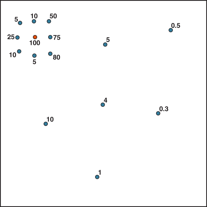
Figure 6-10. Hypothetical exposure area with clustered data.

One approach for estimating the area-weighted average is to use Thiessen polygons (ESRI 2012) to determine the portion of the larger area which is represented by a single sampling location. Thiessen polygon boundaries define the area that is closest to each point relative to all other points; the boundaries are mathematically defined by the perpendicular bisectors (or half-way point) of the lines between all points (NJDEP 2012b). Figure 6-11 depicts the Thiessen polygons constructed for the sampling locations shown in Figure 6-10. These polygons can be developed efficiently using GIS software, but they can also be constructed by simply using a ruler and a pencil.

Additional spatial interpolation methods, such as kriging and nearest-neighbor algorithms, may also be appropriate for supporting the calculation of areal averages. Consult with a risk assessor, however, to determine the applicability of these methods before using them in the evaluation of risk.

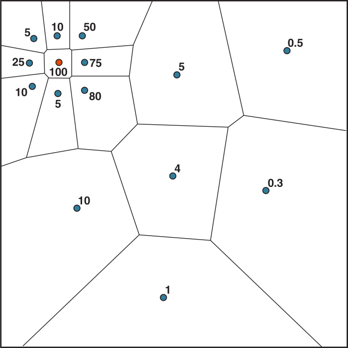
Figure 6-11. Hypothetical one-acre exposure area with Thiessen polygons.

Area-weighted (or spatially weighted) average concentrations for the exposure area can be calculated by weighting concentrations from each location by the area which they represent. The area-weighted average concentration for the exposure area is thus the sum of the products of the chemical concentration and surface area for each individual subarea, divided by the total surface area of the exposure area.

Table 6-1 presents the area-weighted average calculations performed for the hypothetical exposure area presented in Figure 6-10 and Figure 6-11.

For comparison purposes, the 95% UCL on the mean for this data set would be 58 mg/kg.

Statistical methods can assess the uncertainty in area-weighted averages. For example, it would be possible to calculate a 95% UCL on the area-weighted mean by using a nonparametric bootstrap method with weighted bootstrap resampling. With this approach, the bootstrapped data set would consist of a number of draws equal to the total number of original samples in the hypothetical exposure area. The probability of drawing a sample from the original distribution is equal to the Thiessen polygon area divided by the total area of the exposure area to give an area weighting factor. As a result, each data point in the original data set contributes, on average, to the area weighted average according to the relative area that it represents within the exposure area. Bootstrap techniques such as the Efron’s percentile method can be used to establish the lower confidence limit (LCL) and UCL at a particular level of confidence.

6.2.4.3 Option – Composite Samples

Unless carefully designed, collected, and processed, composite samples may dilute or otherwise misrepresent concentrations at specific points. Composite samples, however, may be useful to quantify the mean concentration for nonvolatile chemicals by physically mixing samples to yield an average concentration (USEPA 1989a; USEPA 1996b).

Techniques such as incremental sampling methodology (ISM) offer a structured composite sampling and processing protocol to reduce data variability. This approach can be an appropriate, reliable, and cost-effective means for assessing exposure risk (estimating mean concentration within an exposure area). ISM provides an unbiased estimate of mean chemical concentrations within an exposure unit (ITRC 2012a), rather than simply indicating the presence of individual hot spotsHot spots are considered to be soil volumes with relatively high concentrations that could be present at a site but whose locations and dimensions cannot be anticipated prior to sampling (ITRC 2012a).. This technique is also useful at large sites where relatively similar chemical concentrations are suspected, and at sites where exposure units are well defined and the average concentration across the exposure unit is of interest. ISM is consistent with sampling theory that is long accepted in the mining industry. Currently, ISM is accepted for use in risk assessments by some state agencies, the U.S. Department of Defense, and various USEPA regions.

6.2.4.4 Option – Weighted UCLs on the Mean

Weighted UCLs on the mean can also be used where exposure units are well defined and data for an exposure area are so unevenly distributed that UCLs on the mean do not provide reasonable estimates of the exposure concentration in an exposure area. Consider the example presented in Section 6.2.4.2 and Figure 6-10. In this example, a number of surface soil sample locations are clustered in one corner of the exposure area. One approach to estimate an exposure concentration in this area would be to calculate UCLs on the mean for two subareas of the overall exposure area (Figure 6-12). In Subarea 1, where the data are clustered, a UCL of the mean is calculated. A UCL on the mean is also calculated for Subarea 2. The resulting UCLs on the mean can then be weighted together account for the relative portions of the area over which they are located.

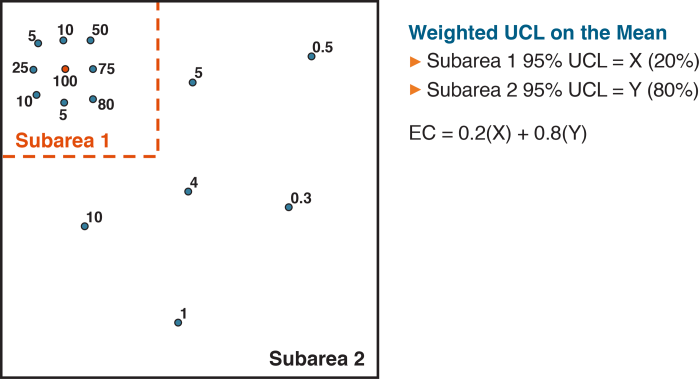
Figure 6-12. Hypothetical exposure subareas.

Environmental data related to natural or anthropogenic background concentrations are commonly either site- or area-specific, or from the literature if site-specific data are not available or practical. Site-specific background concentration data may be the preferred alternative because the relationship of regional or state-wide concentrations to site-specific concentrations can be difficult to establish (see Section 3.3.7 for more information). Published data for background soil concentrations may be obtained from various sources, such as USGS (2012), Dragun and Chekiri (2005), and state-specific publications (see Section 4.5.6).

In some cases background-related risks may not be presented in the risk assessment. This omission may simplify the assessment when initial screening against background concentrations indicates that concentrations of chemicals that significantly affect risk are well above background concentrations, or when no background data are available for chemicals that significantly affect risk. When background concentrations are likely to represent a significant portion of overall risk, risk management decisions may require distinguishing the contribution from background concentrations relative to total site risk. Not considering the contributions from background concentrations can lead to an overestimate of site-related risk, which can result in unnecessary risk management decisions, undue public concern, or distrust of the protectiveness of the remedy.

The decision regarding appropriate options for characterizing risk (including site-related versus background risk) should consider risk communicationRisk communication is the formal and informal process of communication among and between regulatory agencies and organizations responsible for site assessment and management, and the various parties who are potentially at risk from or are otherwise interested in the site. needs. Two options for using and presenting background exposure concentrations and risks versus site-related exposure concentrations and risks are provided below.

6.2.5.1 Option – Present Separate Risk Calculations

One option, which is consistent with recommendations in USEPA’s Role of Background in the CERCLA Cleanup Program (USEPA 2002e), is to “address site-specific background issues at the end of the risk assessment” by distinguishing in the risk characterizationThe risk characterization integrates information from the preceding components of the risk assessment and synthesizes an overall conclusion about risk that is complete, informative and useful for decision makers (USEPA 2000c). “the contribution of background to site concentrations.” With this approach, total and background chemical exposure concentrations are calculated for receptor risk estimates for both background and site-related exposures and included in the risk characterization section of the risk assessment. In this process, consider the following:

• Compare background risks and site risks based on similar sampling designs. Ideally, samples considered in the analysis are collected using the similar sampling design and methods (apples to apples comparison), or at least are considered to be equivalent as to what is represented by the data set (for example, similar sample depths, soil types, native soils versus recent fill placement, soil removal or site regrading). For example, background concentrations should be characterized using  ISM when site data are collected using ISM (ITRC 2012a). Another example is to compare data of the same time series when data may have temporal trends or patterns, which is commonly observed for environmental media such as water or air.
• Use a regulatory definition of background concentration to calculate health risks. Regulatory programs may define regional or statewide background concentrations for certain chemicals. Sometimes these background concentrations are based on risk management considerations to help identify chemicals in environmental media for evaluation in a risk assessment. These defined background concentrations are a convenient screen against calculated risk-based concentrations (back-calculated risk assessment; see Section 2.1). Background risks calculated using these defined concentrations, however, are unlikely to accurately represent background contributions to site risks since they often represent the upper end of the range of possible background concentrations. These values should not be used to estimate background risk because background risk should be based on an estimate of the mean concentration. Instead, add commentary to the risk assessment to note the defined regulatory background concentration for the chemical and its basis, so that this value can be factored into the risk management decision process.

6.2.5.2 Option – Subtract Background Concentrations from Exposure Concentrations

Background concentrations of chemicals may be subtracted from detected concentrations of chemicals at a site. The resulting site-related concentrations could be below the screening value, leading to a decision that the chemical is no longer retained for evaluation in the risk assessment. In these cases, the risks presented then focus on those risks present based on the difference between site and background concentrations. This method is appropriate if the statistical basis for the two data sets are the same and if the same statistical methods are used to analyze both data sets (apples to apples comparison). When subtracting background concentrations, consider the following:

• Subtract a background 95% UCL on the mean concentration from a site 95% UCL on the mean concentration to estimate the site-related concentration. Because the 95% UCL on the mean is a function of sample size and variability in concentrations, both of which may differ between site and background areas, a simple subtraction may not be defensible. In particular, if fewer background samples than site samples are available from an exposure area, the background 95% UCL on the mean may be biased high as compared to the site 95% UCL on the mean, and the site-related risk may be underestimated (not conservative). Conversely, if the background data set is larger than the data set used to calculate a 95% UCL on the mean for the exposure area, then the bias for the 95% UCL on the mean for background may be lower than that of the exposure area UCL on the mean, in which case the mean concentration for the site may be overestimated (overly conservative). Overestimating the exposure area mean concentration may be suitable for purposes of site screening or for remedial decision making, if acceptable to reviewers.
• Subtract background concentrations from site concentrations when their mean concentrations have been estimated using different statistics. For example, subtracting a 95% upper tolerance limit (UTL) of background concentration from an exposure area with a 95% UCL on the mean is not appropriate (apples to oranges comparison). Subtraction may be appropriate if the background and exposure area concentration data sets are analyzed with the same statistical method.